How do you do a Vlookup match?

The primary formula we'll be using is VLOOKUP:

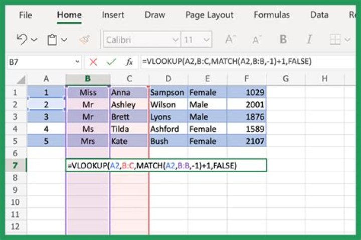
1. =VLOOKUP ( lookup value , table_array , col_index_num , [range_lookup] )
2. To use this formula, you'll need a lookup value and a table array.
3. =MATCH ( lookup value , lookup_array , [match _type] )

Also question is, how do you do a Vlookup with closest match?

The [range_lookup] argument is set to TRUE, which tells the Vlookup function to find the closest match to the lookup_value. I.e. if an exact match is not found, then the function should return the closest value below the lookup_value.

Furthermore, how do I match a column in a Vlookup in Excel? How to Compare Two Columns in Excel

1. Click the Compare two columns worksheet tab in the VLOOKUP Advanced Sample file.
2. Add columns in your workbook so you have space for results.
3. Type the first VLOOKUP formula in cell E2:
4. Click Enter on your keyboard and drag the VLOOKUP formula down through cell C17.

Keeping this in view, how do you use Vlookup correctly?

How to Use VLOOKUP in Excel

1. Identify a column of cells you'd like to fill with new data.
2. Select 'Function' (Fx) > VLOOKUP and insert this formula into your highlighted cell.
3. Enter the lookup value for which you want to retrieve new data.
4. Enter the table array of the spreadsheet where your desired data is located.

What is the difference between match and Vlookup?

The key difference between INDEX MATCH and VLOOKUP is that VLOOKUP requires a static column reference while INDEX MATCH uses a dynamic column reference. With VLOOKUP, most people will input a specific, static number to indicate which column they want to return from.

Related Question Answers

Which is better index match or Vlookup?

With unsorted data, VLOOKUP and INDEX-MATCH have about the same calculation times. With sorted data and an approximate match, INDEX-MATCH is about 30% faster than VLOOKUP. With sorted data and a fast technique to find an exact match, INDEX-MATCH is about 13% faster than VLOOKUP.

How do I do a dynamic Vlookup in Excel?

If you ever work with large tables of data and you want to insert a VLOOKUP formula that dynamically updates to the next column as you copy it across, then the VLOOKUP with the COLUMNS function is what you need.

Can you use Vlookup with IF function?

One of the most common scenarios when you combine If and Vlookup together is to compare the value returned by Vlookup with a sample value and return Yes / No or True / False as the result. Translated in plain English, the formula instructs Excel to return True if Vlookup is true (i.e. equal to the sample value).

Can you use Vlookup for 2 columns?

However, tweaking the formula allows us to use VLOOKUP to look across multiple columns. VLOOKUP doesn't handle multiple columns. You can find matches for Movie and Showtime columns individually but to find a match based on both the columns, you would need to modify the VLOOKUP formula.

How do I match data in Excel?

Compare Two Columns and Highlight Matches

1. Select the entire data set.
2. Click the Home tab.
3. In the Styles group, click on the 'Conditional Formatting' option.
4. Hover the cursor on the Highlight Cell Rules option.
5. Click on Duplicate Values.
6. In the Duplicate Values dialog box, make sure 'Duplicate' is selected.

How do I close a match in Excel?

Closest Match

1. The ABS function in Excel returns the absolute value of a number.
2. To calculate the differences between the target value and the values in the data column, replace C3 with C3:C9.
3. To find the closest match, add the MIN function and finish by pressing CTRL + SHIFT + ENTER.

When would you use true in a Vlookup?

A parameter of FALSE means that VLOOKUP is looking for an EXACT match for the value of 10251. A parameter of TRUE means that a "close" match will be returned. Since the VLOOKUP is able to find the value of 10251 in the range A1:A6, it returns the corresponding value from B1:B6 which is Pears.

How accurate is Vlookup true?

VLOOKUP results with TRUE after the data has been sorted in Excel 2007 and Excel 2010. This in fact is not an incorrect result at all as we were using TRUE, which returns the exact result OR the nearest result it can find (the next largest when working with numbers).

Does Google sheets do Vlookup?

Google Sheets VLOOKUP function can be used to look for a value in a column and when that value is found, return a value from the same row from a specified column. That's exactly how Google Sheets VLOOKUP function works.

How does excel approximate match work?

The approximate match returns the next largest value that is less than your specific lookup value. 3. To use the vlookup function to get an approximate match value, your first column in the table must be sorted in ascending order, otherwise it will return a wrong result.

How does excel calculate approximate match?

In the first step, the match, Excel must find the matching value. You tell Excel the value to find, such as “ABC Company” and you tell Excel where to look, such as in a range of cells. You are asking Excel to find the lookup value in the lookup range. Step two, the return, is the function's result.

How do you create a Fuzzy Lookup in Excel?

We do this by clicking on the File tab, and then selecting Options/Add-Ins. In the menu below, select the COM Add-Ins option, and then in the window that appears, select the option to activate. If you've done everything right, a new ribbon wil appear that contains only one option will appear – Fuzzy Lookup!

What is Ctrl Shift Enter in Excel?

When you press Ctrl+Shift+Enter, Excel surrounds the formula with braces ({ }) and inserts an instance of the formula in each cell of the selected range.

What is Vlookup in simple words?

VLOOKUP stands for 'Vertical Lookup'. It is a function that makes Excel search for a certain value in a column (the so called 'table array'), in order to return a value from a different column in the same row.

What is Vlookup in Excel with example?

The VLOOKUP function always looks up a value in the leftmost column of a table and returns the corresponding value from a column to the right. 1. For example, the VLOOKUP function below looks up the first name and returns the last name. No worries, you can use INDEX and MATCH in Excel to perform a left lookup.

How do you do a Vlookup on sheets?

In your Google Sheet, click Add-ons > Multiple VLOOKUP Matches > Start, and define the lookup criteria:

1. Select the range with your data (A1:D9).
2. Specify how many matches to return (all in our case).
3. Choose which columns to return the data from (Item, Amount and Status).
4. Set one or more conditions.

How do I compare two lists in Excel?

Compare Two Lists

1. First, select the range A1:A18 and name it firstList, select the range B1:B20 and name it secondList.
2. Next, select the range A1:A18.
3. On the Home tab, in the Styles group, click Conditional Formatting.
4. Click New Rule.
5. Select 'Use a formula to determine which cells to format'.
6. Enter the formula =COUNTIF(secondList,A1)=0.

Where is Vlookup in Excel?

How to use VLOOKUP in Excel

1. Click the cell where you want the VLOOKUP formula to be calculated.
2. Click "Formula" at the top of the screen.
3. Click "Lookup & Reference" on the Ribbon.
4. Click "VLOOKUP" at the bottom of the drop-down menu.
5. Specify the cell in which you will enter the value whose data you're looking for.

How do I do a Vlookup on multiple sheets?

How to use the formula to Vlookup across sheets

1. Write down all the lookup sheet names somewhere in your workbook and name that range (Lookup_sheets in our case).
2. Adjust the generic formula for your data.
3. Enter the formula in the topmost cell (B2 in this example) and press Ctrl + Shift + Enter to complete it.

Can Vlookup return text?

Can VLOOKUP work with text as well as numbers? Yes. VLOOKUP can search for textual values just as well as it can search for numbers. The example above would search for the product names, which are text rather than numbers.

How do you sum a Vlookup?

Vlookup is a very versatile function which can be combined with other functions to get some desired result, one such situation is to calculate the sum of the data ( in numbers) based on the matching values, in such situations we can combine sum function with vlookup function, the method is as follows =SUM(Vlookup(

Can you use Sumif and Vlookup together?

The tasks may vary, but the essence is the same - you want to look up and sum values with one or several criteria in Excel. You can work out a solution by combining Excel's VLOOKUP or LOOKUP with SUM or SUMIF functions.

How do I do a Vlookup formula in multiple columns?

The VLOOKUP function can be combined with other functions such as the Sum, Max or Average to calculate values in multiple columns. As this is an array formula, to make it work we simply need to press CTRL+SHIFT+ENTER at the end of the formula.